Split the US mainland map into grids.

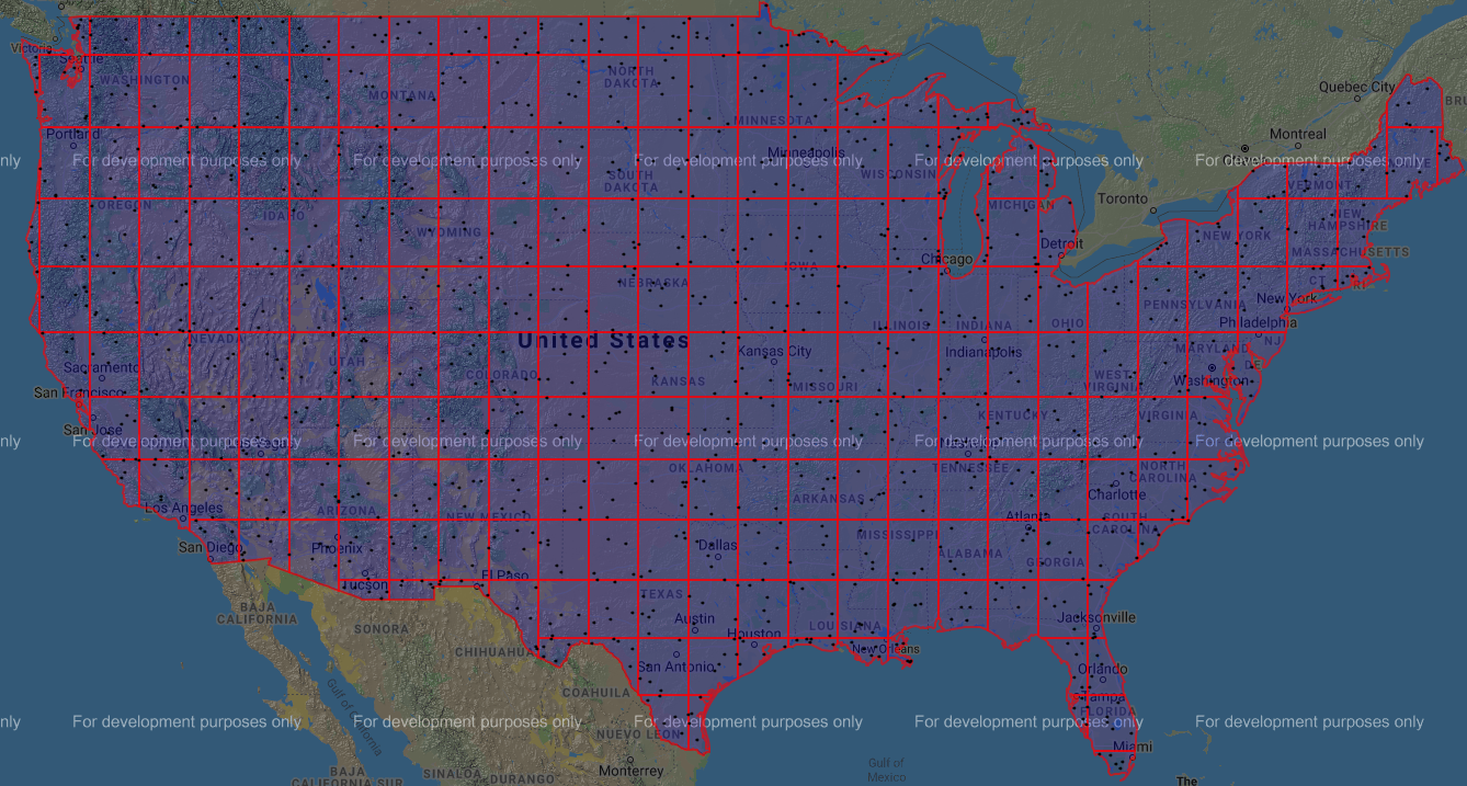
The shape file of the US provided by the United States Census Bureau was used. The shapefile coordinates were converted into polygons and the polygon for mainland USA was extracted. Shapely was used for all geometry related tasks. For this project, we focused only on the mainland boundaries. A mesh of square boxes were overlayed on the USA polygon and the squares were clipped at the polygon boundaries to create grids of the US polygon. Each grid had a maximum area of 4 sq. units totaling 138.265 sq units, with the grids at borders being smaller. Smaller grids (less that 0.1 times area of the largest grids) were combine with the neighboring grids to avoid some grids having no data. This process resulted in 243 grids forming the mainland US.

Scraped Google street view data from multiple locations in each grid.

Three images were collected per location for 40 locations per grid using the Google Street View static API. Each of the 3 images represented headings of 0 degrees, 90 degrees and 180 degrees of a particular location. The 243 grids thus resulted in 9720 location data points and 29160 images. Each image is of 30 KB resulting in 0.8 GB of data. The price of each image was $0.007 totaling $204

Images under a given lat/long were stored in the folder: "grid-number+latitude,longitude" and the images in them were stored under the filename: "number-image-date.jpg". 3 images for the lat/long 42.77, -124.06 were for example stored in the filepath: "dataCombined/0+42.775957,-124.0667758/0-2009-07.jpg". The 9720 data points that collected were split into 8748 training and 972 testing points. About 90 percent of the data was reserved for training and 10 percent for testing.

Built and trained two custom CNN/LSTM using Keras

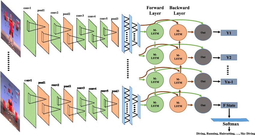
The input images were loaded and converted to numpy arrays using the tf.keras.preprocessing.image.loadimg function. The array was made up of rgb values and had the following shape (300, 600, 3). Since the input consists of three such images, the shape of each training input turned into (3, 300, 600, 3). The model used a soft-maxed output for prediction. Therefore for training, the grid numbers corresponding to given input image vector were converted to one hot vectors. This was done using the tf.keras.utils.tocategorical function. The one hot output vector had a shape of (243,). Two models were trained to compare the performance. The first model had a ResNet CNN whose weights were frozen during training connected to a trainable LSTM to process the sequence of three images at a time. The next model had a trainable CNN connected to an LSTM. The models were trained in batches of 300 input vectors using Google Colab GPUs.

Ran predictions and scored models on test dataset.

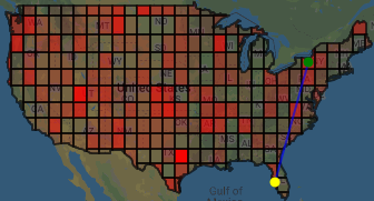
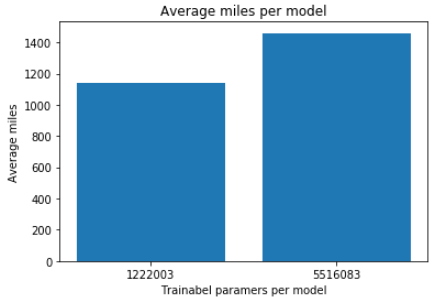
Python google maps API gmaps was used to visualize a single soft-maxed prediction across all grids. The opacity of each grid polygon is set to the weight of that index in the array of soft-maxed prediction probabilities. As seen in the figure different opacity of reds scaled between values of 0 to 1 according to prediction confidence. The actual location grid is denoted by a green point and the predicted grid (grid with the highest score) a yellow point. The distance between these points is calculated using haversine distance. This distance is used to draw a line between the start and end points which is seen in the figure as the blue line. The haversine distance between predicted and actual locations were calculated for the entire test set were calculated and the average was taken to get a score for the model. The score represents the average distance in miles the model was wrong by. The difference in predictions scores between the two models are shown.

The similarity in street view images across different parts of mainland united states, could be one of the reason for our model's poor performance. The was a reduction in error (distance) while training the model for 30 epochs on just 300 images. Insted of using just street view images, diversity of images could be improved by adding prominent landmarks, features unique to a given grid for future work. Another noteworthy fact is that human players of the game geoguessr are allowed to walk around (specific number of steps) using google street view. If the model was allowed to do the same and collected data as a larger stream of images per location, there could be a performance improvement with the model learning more about a location just like a human player.

Development was done in Python. Jupyter notebook was used for testing and development. Keras was used to build and train machine learning models. Google Colab GPU infrastructure was used for training.